From the previous lesson, we have already introduced motions with quantifiable velocities, such as constant velocities and average velocities. Moving on, this section will introduce varying velocities as a result of acceleration. But before we begin, let us define acceleration.
If you are travelling at a rate of 50 m/s, then after a second your rate increases to 60 m/s, and 70 m/s after the next second (Figure 1). This indicates that you are increasing your pace as time passes or that you are “accelerating.’’ According to our example, you are accelerating at a rate of 10 m/s per second, which is expressed as 10 m/s/s or 10 $\mathrm{m/s^2}$. With this, we can now define acceleration mathematically. It is the change in velocity with respect to time. Thus, acceleration can be denoted as,
$$\begin{align} \vv{a}=\frac{\Delta\vv{v}}{t}=\frac{\vv{v_f}-\vv{v_i}}{t} \label{eq:uniform accelerated motion 1} \end{align}$$
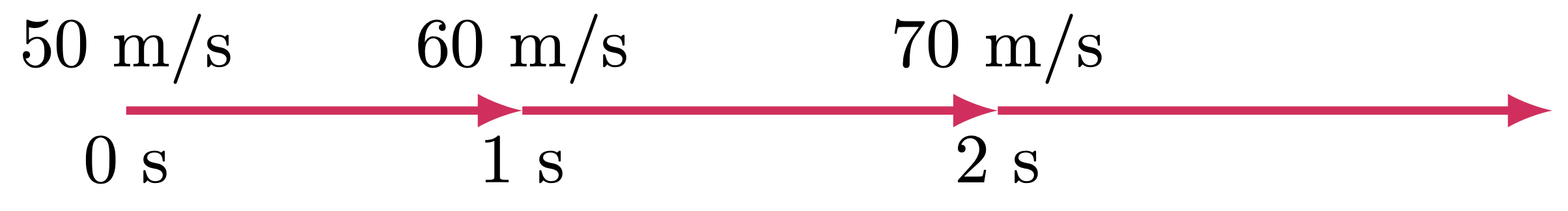
Figure 1: Accelerating at $10\un{m/s^2}$
Kinematic Equations
There are four well-known kinematic equations for uniformly accelerated motion. They are as follows:
$$\begin{align} v_f = v_i+at \label{eq:kinematic eqn 1} \\ \Delta s = \br{ \frac{v_i+v_f}{2} }t \label{eq:kinematic eqn 2} \\ \Delta s = v_it+\frac{1}{2}at^2 \label{eq:kinematic eqn 3} \\ {v_f}^2 = {v_i}^2+2a\Delta s \label{eq:kinematic eqn 4} \end{align}$$
These equations are derived from $\eref{eq:uniform accelerated motion 1}$ and other equations that we’ve already discussed from the previous lesson. And these four equations will be used in solving problems that have a uniform acceleration, may it be increasing or decreasing.
Take note that if an object is decelerating, then its acceleration is negative “$-a$,’’ and if an object starts from rest then the initial velocity is zero. Similarly, if an object is dropped, the initial velocity is also zero.
Derivation of the kinematic equations
By now, we are already familiar that most formulas are just derived from simpler formulas that bear simpler notions. The kinematic equations are not excluded from that idea, these four equations are all derived formulas. To start, let us derive the first equation.
$\typB{Proof of Equation \ref{eq:kinematic eqn 1}},$
This first equation can be attained by just rearranging $\eref{eq:uniform accelerated motion 1}$,
\[\begin{align*} a &= \frac{v_f-v_i}{t} \\ at &= v_f-v_i \\ v_f &= v_i + at \tagans \end{align*}\]$\typB{Proof of Equation \ref{eq:kinematic eqn 2}},$
In this equation, we will need to start from an equation that we have learned from our previous lesson. If you could recall the formula for the magnitude of average velocity,
\[\begin{align*} \bar{v} &= \frac{\Delta s}{\Delta t} \\ \end{align*}\]Then rearranging the equation to express the displacement explicitly,
\[\begin{align*} \Delta s &= \bar{v} \Delta t \end{align*}\]We can substitute the average velocity with $\frac{v_i + v_f}{2}$ since the average of two values can be established through adding those values then dividing the sum to the number of given values, which in this case, is 2.
\[\begin{align*} \Delta s &= \br{\frac{v_i + v_f}{2}} \Delta t \end{align*}\]Given that $t$ is the time ellapsed, we can express the equation as,
\[\begin{align*} \Delta s &= \br{\frac{v_i + v_f}{2}} t \end{align*}\]$\typB{Proof of Equation \ref{eq:kinematic eqn 3}},$
To derive the third kinematic equation, we need to use both $\eref{eq:kinematic eqn 1}$ and $\eref{eq:kinematic eqn 2}$. Starting with our recently derived equation,
\[\begin{align*} \Delta s &= \br{\frac{v_i + v_f}{2}} t \end{align*}\]Then using $\eref{eq:kinematic eqn 1}$, we can substitute the final velocity wth $v_i + at$.
\[\begin{align*} \Delta s &= \br{\frac{v_i + v_i + at}{2}} t \\ &= \br{\frac{2v_i + at}{2}} t \\ &= \br{v_i + \frac12at} t \\ &= v_i t + \frac12at^2 \end{align*}\]$\typB{Proof of Equation \ref{eq:kinematic eqn 3}},$
For the last kinematic equation, we will start with $\eref{eq:kinematic eqn 2}$,
\[\begin{align*} \Delta s &= \br{\frac{v_i + v_f}{2}} t \end{align*}\]As you may have observed, there is no variable $t$ in the fourth equation. Thus, to eliminate the variable, we must express $t$ with different variables. In this scenario, we can use $\eref{eq:kinematic eqn 1}$ and explicitly define $t$ in the equation.
\[\begin{align*} v_f &= v_i + at \\ t &= \frac{v_f - v_i}{a} \end{align*}\]Then substituting $t$ to the first equation gives us,
\[\begin{align*} \Delta s &= \br{\frac{v_i + v_f}{2}} \br{\frac{v_f - v_i}{a}} \\ &= \frac{ {v_f}^2-{v_i}^2 }{2a} \\ 2a\Delta{s} &= {v_f}^2-{v_i}^2 \\ {v_f}^2 &= {v_i}^2 + 2a\Delta{s} \end{align*}\]However, you may wonder why these formulas exist since we can just derive them using basic formulas. As you may have noticed, each formula contains a unique combination of variables. Thus, depending on the parameters given on a problem, using one formula than another can simplify the solution.
By enumerating all variables in the kinematic equations, we obtain the following: $v_i$, $v_f$, $a$, $t$, and $s$. While all four equations contain a total of five (5) variables, each kinematic equation contains only four (4) variables. Thus, determining the missing variable can provide insight into the equation we will use to solve the problem. Tabulating this information provides us with,
Table 1: Missing variables in kinematic equations
$\example{1}$ A car overtaking a truck, uniformly accelerates its speed from 40 kph to 90 kph in 8 seconds. Calculate (a) the average velocity in m/s, (b) the car’s acceleration in $\mathrm{m/s^2}$, and (c) the distance travelled during the 8 second period in meters.
$\solution$
$\given$
\(\begin{align*}
v_i &= 40\un{kph} & \\
v_f &= 90\un{kph} \\
t &= 8\un{s}
\end{align*}\)
$\For{a}$
In uniform accelerated motion, to determine for the average velocity, add the initial and final velocities then divide by 2.
$\For{b}$
Given that $v_i$, $v_f$, and $t$ are all provided, and only $a$ is required. In this particular problem, the variable $s$ is missing. Thus, utilizing Table 1 indicates that the simplest solution is to use $\eref{eq:kinematic eqn 1}$. Hence,
$\For{c}$
In this problem, we could now use any of the kinematic equations since we already have solved for the different parameters. However, there are instances when we are uncertain about our answers. Thus, if possible, it would be prudent to solve the problem using the provided parameters. $v_i$, $v_f$, and $t$ are all specified in this example, while $\Delta{s}$ is required. Consequently, the variable $a$ is missing. Hence, the simplest approach, as determined by Table 1, is to use $\eref{eq:kinematic eqn 2}$.
Since $\overline{v}=\frac{v_i+v_f}{2}$,
\[\begin{align*} \Delta s &= \overline{v}t \\ &= (18.06 \un{m/s})(8 \un{sec}) \\ &= 144.48 \un{m} \tagans \end{align*}\]